Analytical comparisons
This section presents comparisons between analytical solutions and modelled solutions using gprMax.
Hertzian dipole in free space
This example is of a Hertzian dipole, i.e. an additive source (electric current density), in free space.
1#title: Hertzian dipole in free-space
2#domain: 0.100 0.100 0.100
3#dx_dy_dz: 0.001 0.001 0.001
4#time_window: 3e-9
5
6#waveform: gaussiandot 1 1e9 myWave
7#hertzian_dipole: z 0.050 0.050 0.050 myWave
8#rx: 0.070 0.070 0.070
The function hertzian_dipole_fs, which can be found in the analytical_solutions module in the tests sub-package, computes the analytical solution.
Results
図 46 shows the time history of the electric and magnetic field components of the modelled and analytical solutions. The responses completely overlap one another due to their similarity. Therefore, 図 47 shows the percentage differences between the modelled and analytical solutions.
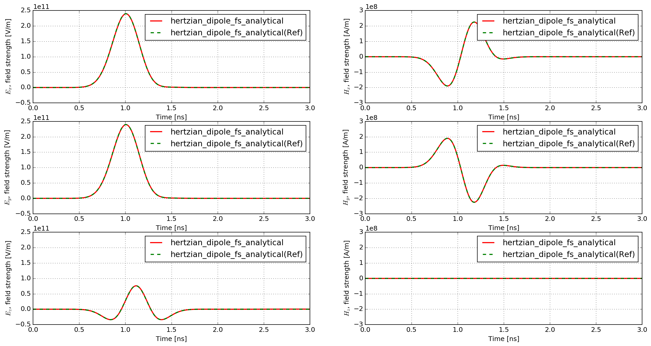
図 46 Time history of the electric and magnetic field components of the modelled and analytical solutions ('Ref', in this case, indicates solution calculated from theory).
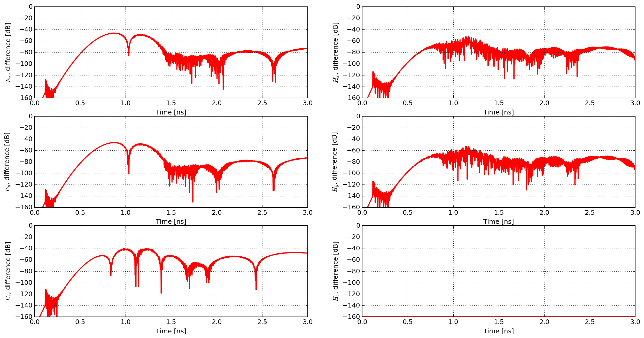
図 47 Percentage differences between the modelled and analytical solutions.
The match between the analytical and numerically modelled solutions is excellent. The maximum difference is approximately 1%, which is observed in the Ez field component (the same direction as the Hertzian dipole source). The other electric field components exhibit maximum differences of approximately 0.5%, and the magnetic field components 0.25%.
Half-wave dipole in free space
See the section on antenna example models for the simulated s11 parameter and input impedance of a half-wave dipole antenna in free space. The resonant frequency and input impedance from the model agree very well with the theoretical predictions for a half-wave dipole antenna.